I am creating a supplies list for work. It has multiple sheets for each department. The first sheet is a master list which will be where I manually enter all supplies, product numbers, manufacturer, reference ID, etc... I want the following sheets to pull off this main list the information of the supplies specific only to each department automatically. Is there a way to create a formula that will perform such a task?

If your first column of the master list is some sort of unique ID that you can enter into cell on the other departmental sheets, then you could use a formula like

=VLOOKUP($A2,'Master List'!$A:$Z, COLUMN(B2), False)

copied to the right (and down, for other ID numbers) to pull all the information for each ID.

Thank you for responding Bernie. Sorry, I have been trying to get my account verified so I can post an example of what I'm trying to do with a screen shot. I am having trouble with exactly what info goes where. Once I get my account verified then I will be able to display my example.

 I do not know exactly what information to place where so if you could further elaborate after reviewing the below example...

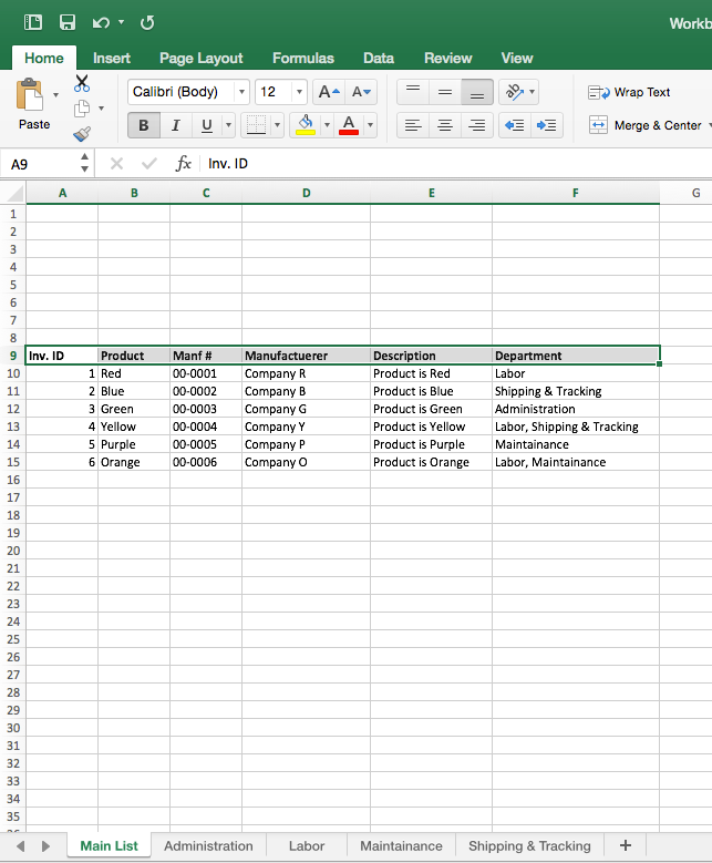
I want the 'Main List' as a master where I will place all information and add future information...I would like a formula that would pull all the information for products that pertain to specific departments to their dedicated sheets...for instance looking at Column (F) it has what departments each product is under some products fall under more then 1 department so I would want it pulled to both for instance row (6) to sheets labeled 'Labor' and 'Maintenance'. I would want all information in that row to follow exactly as shown off the 'Main List' though...and looking at Inv. ID I did label 1-6 but they will in fact be randomly assigned 6-7 digit numbered codes for each supply item so I apologize for that...I would like the =vlookup function to search for the department then pull the entire row's information to the appropriate sheet.

I hope that may make what I am asking a little more clear. It took me a while as I first had to look up a forum to attach the screenshot and create a photo bucket acct then get verified.

OK. On your other sheets - let's start with Administration (but all the others will be similar) - enter Administration into cell A2. Then in A3:E3, enter the headers that you have in A9:E9 of sheet "Main List".  Then, in cell A4, array enter - Enter using Strl-Shift-Enter instead of just Enter - the formula

=IF(COUNTIF('Main List'!$F:$F,"*"&$A$2&"*")>=ROWS($A$1:$A1),INDEX('Main List'!$A:$F,LARGE(ISNUMBER(SEARCH($A$2,'Main List'!$F$1:$F$2000))*ROW($A$1:$A$2000),COUNTIF('Main List'!$F:$F,"*"&$A$2&"*")-(ROWS($A$1:A1)-1)),COLUMN(A1)),"")

and copy to B4:E4, and copy A4:E4 down until the formulas return blanks.  Do the same for the other department sheets, and you're done.

• Edited by Bernie Deitrick, Excel MVP 2000-2010Microsoft community contributor 12 hours 43 minutes ago
• Marked as answer by JJ_RN 9 hours 47 minutes ago

OMG Thank you soooooo much Bernie!!! I have applied it to my actual workbook and it is saving me thousands of entries!!

OK. On your other sheets - let's start with Administration (but all the others will be similar) - enter Administration into cell A2. Then in A3:E3, enter the headers that you have in A9:E9 of sheet "Main List".  Then, in cell A4, array enter - Enter using Strl-Shift-Enter instead of just Enter - the formula

=IF(COUNTIF('Main List'!$F:$F,"*"&$A$2&"*")>=ROWS($A$1:$A1),INDEX('Main List'!$A:$F,LARGE(ISNUMBER(SEARCH($A$2,'Main List'!$F$1:$F$2000))*ROW($A$1:$A$2000),COUNTIF('Main List'!$F:$F,"*"&$A$2&"*")-(ROWS($A$1:A1)-1)),COLUMN(A1)),"")

and copy to B4:E4, and copy A4:E4 down until the formulas return blanks.  Do the same for the other department sheets, and you're done.

• Edited by Bernie Deitrick, Excel MVP 2000-2010Microsoft community contributor Friday, July 17, 2015 6:48 PM
• Marked as answer by JJ_RN Friday, July 17, 2015 9:44 PM

OK. On your other sheets - let's start with Administration (but all the others will be similar) - enter Administration into cell A2. Then in A3:E3, enter the headers that you have in A9:E9 of sheet "Main List".  Then, in cell A4, array enter - Enter using Strl-Shift-Enter instead of just Enter - the formula

=IF(COUNTIF('Main List'!$F:$F,"*"&$A$2&"*")>=ROWS($A$1:$A1),INDEX('Main List'!$A:$F,LARGE(ISNUMBER(SEARCH($A$2,'Main List'!$F$1:$F$2000))*ROW($A$1:$A$2000),COUNTIF('Main List'!$F:$F,"*"&$A$2&"*")-(ROWS($A$1:A1)-1)),COLUMN(A1)),"")

and copy to B4:E4, and copy A4:E4 down until the formulas return blanks.  Do the same for the other department sheets, and you're done.

• Edited by Bernie Deitrick, Excel MVP 2000-2010Microsoft community contributor Friday, July 17, 2015 6:48 PM
• Marked as answer by JJ_RN Friday, July 17, 2015 9:44 PM

Just curious Bernie, is there a way to make that formula also pull a hyperlink as well? All the data pulls just fine but the beginning of each row has a hyperlink to a photograph of the product and I would like to see if it is possible to have that auto populate to the other sheets as well.

A lot depends on how the hyperlinks are entered.  First, try just wrapping the function in a hyperlink function (but just for the first column).  Array entered (enter using ctrl-shift-enter):

=HYPERLINK(IF(COUNTIF('Main List'!$F:$F,"*"&$A$2&"*")>=ROWS($A$1:$A1),INDEX('Main List'!$A:$F,LARGE(ISNUMBER(SEARCH($A$2,'Main List'!$F$1:$F$2000))*ROW($A$1:$A$2000),COUNTIF('Main List'!$F:$F,"*"&$A$2&"*")-(ROWS($A$1:A1)-1)),COLUMN(A1)),""))

Ok, I tried adding =HYPERLINK to the beginning of the formula. It gave me an error message that corrected on its own but when I try to click on the "link" it gives me a message displayed "cannot open specified file".

I am inserting Hyperlinks to each product by right clicking on the specified cell and adding hyperlink to the picture file. I am guessing this has a different effect based on the first sentence of your response.

Yes - you may need to insert a new column B and use the hyperlink address as the text of that column and base your =HYPERLINK() on that column. You can make the column very narrow or even hide it - just change the COLUMN(A1) to COLUMN(B1) in your formula - the F:F address should auto-update when you insert the new column B.

• Edited by Bernie Deitrick, Excel MVP 2000-2010Microsoft community contributor 15 hours 0 minutes ago